5. Deconvolution in the frequency domain
[1]:
%matplotlib inline
[2]:
from meas_data_preprocessing import *
from hydrophone_data_preprocessing import *
from PyDynamic.uncertainty.propagate_DFT import DFT_deconv, GUM_iDFT
Load calibration data
[3]:
meas_scenario = 13
infos, measurement_data = read_data(meas_scenario=meas_scenario)
_, hyd_data = read_calib_data(meas_scenario=meas_scenario, do_plot=False)
Checking if file ../datasets/pD7_MH44.DAT is already present or download it from https://raw.githubusercontent.com/Ma-Weber/Tutorial-Deconvolution/master/MeasuredSignals/pD-Mode%207%20MHz/pD7_MH44.DAT otherwise:
Replace is False and data exists, so doing nothing. Use replace=True to re-download the data.
Checking if file ../datasets/pD7_MH44r.DAT is already present or download it from https://raw.githubusercontent.com/Ma-Weber/Tutorial-Deconvolution/master/MeasuredSignals/pD-Mode%207%20MHz/pD7_MH44r.DAT otherwise:
Replace is False and data exists, so doing nothing. Use replace=True to re-download the data.
Checking if file ../datasets/MW_MH44ReIm.csv is already present or download it from https://raw.githubusercontent.com/Ma-Weber/Tutorial-Deconvolution/master/HydrophoneCalibrationData/MW_MH44ReIm.csv otherwise:
Replace is False and data exists, so doing nothing. Use replace=True to re-download the data.
The file ../datasets/pD7_MH44.DAT was read and it contains 2500 data points.
The time increment is 2e-09 s
Checking if file ../datasets/pD7_MH44.DAT is already present or download it from https://raw.githubusercontent.com/Ma-Weber/Tutorial-Deconvolution/master/MeasuredSignals/pD-Mode%207%20MHz/pD7_MH44.DAT otherwise:
Replace is False and data exists, so doing nothing. Use replace=True to re-download the data.
Checking if file ../datasets/pD7_MH44r.DAT is already present or download it from https://raw.githubusercontent.com/Ma-Weber/Tutorial-Deconvolution/master/MeasuredSignals/pD-Mode%207%20MHz/pD7_MH44r.DAT otherwise:
Replace is False and data exists, so doing nothing. Use replace=True to re-download the data.
Checking if file ../datasets/MW_MH44ReIm.csv is already present or download it from https://raw.githubusercontent.com/Ma-Weber/Tutorial-Deconvolution/master/HydrophoneCalibrationData/MW_MH44ReIm.csv otherwise:
Replace is False and data exists, so doing nothing. Use replace=True to re-download the data.
[4]:
# metadata for chosen measurement scenario
for key in infos.keys():
    print("%20s: %s" % (key, infos[key]))
                   i: 13
       hydrophonname: GAMPT MH44
     measurementtype: Pulse-Doppler-Mode 7 MHz
     measurementfile: ../datasets/pD7_MH44.DAT
           noisefile: ../datasets/pD7_MH44r.DAT
         hydfilename: ../datasets/MW_MH44ReIm.csv
Pre-process measurement data
[5]:
# remove DC component
measurement_data = remove_DC_component(measurement_data)
[6]:
# Calculate measurement uncertainty from noise data
measurement_data = uncertainty_from_noisefile(infos, measurement_data, do_plot=False)
The file "../datasets/pD7_MH44r.DAT" was read and it contains 2500 data points
[7]:
# calculate spectrum
measurement_data = calculate_spectrum(measurement_data, do_plot=False)
[8]:
# available measurement data
for key in measurement_data.keys():
    print("%12s: %s" % (key, type(measurement_data[key])))
        name: <class 'str'>
     voltage: <class 'numpy.ndarray'>
        time: <class 'numpy.ndarray'>
 uncertainty: <class 'numpy.ndarray'>
   frequency: <class 'numpy.ndarray'>
    spectrum: <class 'numpy.ndarray'>
     varspec: <class 'numpy.ndarray'>
Pre-process calibration data
[9]:
# reduce frequency range of calibration data
hyd_data = reduce_freq_range(hyd_data, fmin=1e6, fmax=100e6)
[10]:
# align spectrum of hydrophone frequency response with spectrum of measurement
fmeas = measurement_data["frequency"].round()
hyd_interp = interpolate_hyd(hyd_data, fmeas)
Deconvolution in the frequency domain
[11]:
# prepare matrix-vector notation for DFT_deconv
H_RI = np.r_[hyd_interp["real"], hyd_interp["imag"]]
U_HRI = np.r_[
    np.c_[np.diag(hyd_interp["varreal"]), hyd_interp["cov"]],
    np.c_[hyd_interp["cov"], np.diag(hyd_interp["varimag"])],
]

# application of DFT_deconv
deconv = {"frequency": measurement_data["frequency"]}
deconv["P"], deconv["U_P"] = DFT_deconv(
    H_RI, measurement_data["spectrum"], U_HRI, measurement_data["varspec"]
)
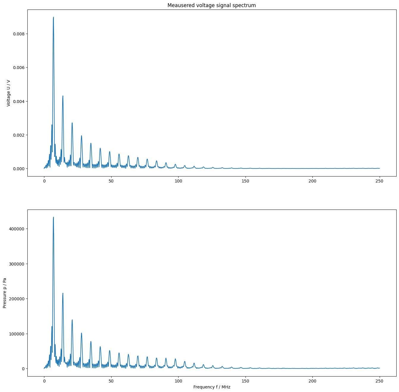
[12]:
f = measurement_data["frequency"]
N = len(f) // 2
figure(figsize=(16, 16))
subplot(2, 1, 1)
plot(f[:N] / 1e6, amplitude(measurement_data["spectrum"]))
title("Meausered voltage signal spectrum")
ylabel("Voltage U / V")

subplot(2, 1, 2)
plot(f[:N] / 1e6, amplitude(deconv["P"]))
xlabel("Frequency f / MHz")
ylabel("Pressure p / Pa")
show()
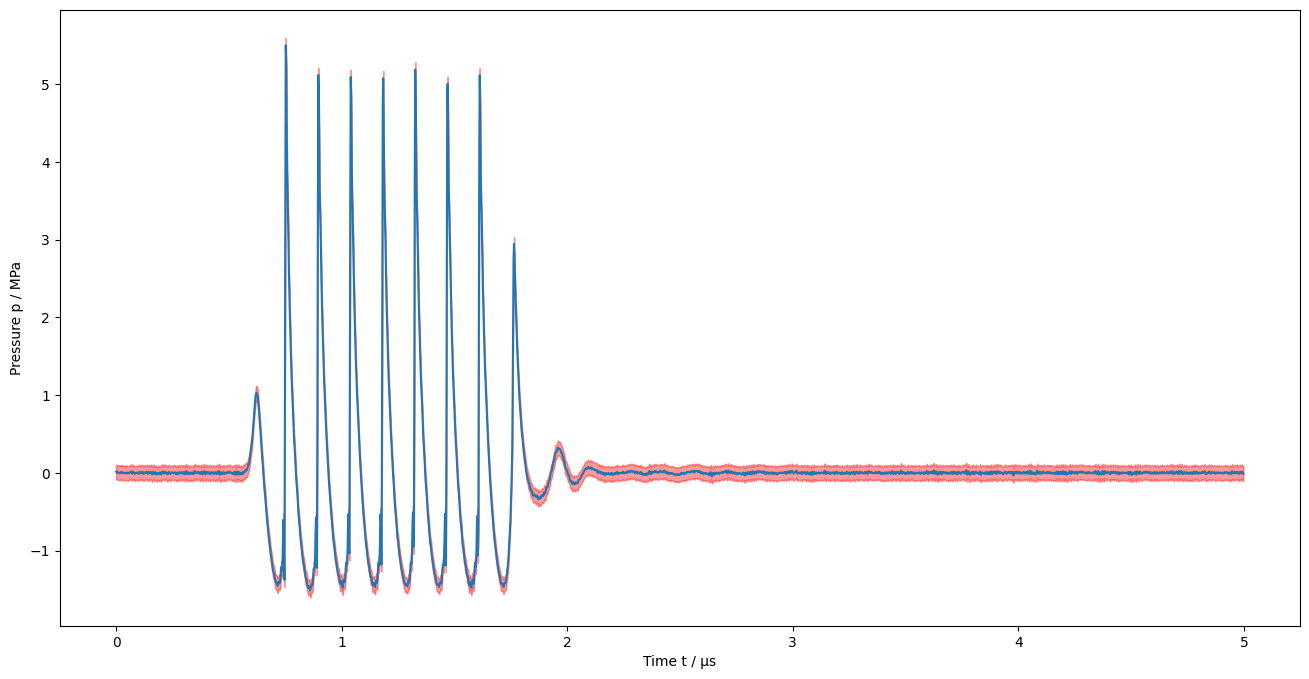
Transformation to the time domain
[13]:
deconvtime = {"t": measurement_data["time"]}
deconvtime["p"], deconvtime["Up"] = GUM_iDFT(deconv["P"], deconv["U_P"])

# correct for normalisation
deconvtime["p"] = deconvtime["p"] / 2 * np.size(deconvtime["t"])
deconvtime["Up"] = deconvtime["Up"] / 4 * np.size(deconvtime["t"]) ** 2
[14]:
figure(figsize=(16, 8))
plot(deconvtime["t"] / 1e-6, deconvtime["p"] / 1e6)
fill_between(
    deconvtime["t"] / 1e-6,
    deconvtime["p"] / 1e6 - 2 * np.sqrt(np.diag(deconvtime["Up"])) / 1e6,
    deconvtime["p"] / 1e6 + 2 * np.sqrt(np.diag(deconvtime["Up"])) / 1e6,
    color="red",
    alpha=0.4,
)
xlabel("Time t / µs")
ylabel("Pressure p / MPa")
show()